Deep Dive into the Heart of Node.js


Every experienced Node.js developer has been there. An application runs smoothly in development, but under the strain of production traffic, a mysterious performance bottleneck appears. The usual toolkit of console.log statements and basic profilers points to no obvious culprit in the application logic. The code seems correct, yet the application slows to a crawl. In these moments, it becomes clear that the problem isn’t just what our code does, but how Node.js is executing it. This is where a surface-level understanding is no longer enough. To solve the hard problems and build truly high-performance applications, we need to look under the hood.


The V8 Engine – The Turbocharged Heart of Execution

While we write our applications in JavaScript, the computer’s processor doesn’t understand functions or objects. It understands machine code. The task of bridging this gap falls to the V8 JavaScript Engine, the same high-performance engine that powers Google Chrome. V8’s primary job is to take our JavaScript and compile it into optimized machine code at lightning speed, making Node.js applications not just possible, but incredibly fast. To achieve this feat, V8 employs a series of sophisticated strategies, beginning with its core component: the Just-In-Time (JIT) compilation pipeline.

The JIT (Just-In-Time) Compilation Pipeline

At the core of V8’s performance is a sophisticated Just-In-Time (JIT) compilation strategy. Instead of fully compiling all JavaScript to machine code before running it (which would be slow to start) or interpreting it line-by-line (which would be slow to run), V8 does both. This process involves a dynamic duo: a fast interpreter named Ignition and a powerful optimizing compiler named TurboFan.Let’s explore this pipeline through the lens of a car rental application. When our Node.js server starts, it needs to be ready for requests immediately. This is where Ignition, the interpreter, shines. Imagine a function that calculates the base cost of a rental:

function calculateBasePrice(car, days) {
// A simple price calculation
return car.dailyRate * days;
}

When this function is defined and first called, Ignition acts like a simultaneous translator. It doesn’t waste time with deep analysis; it quickly converts the JavaScript into bytecode—a low-level, platform-independent representation of the code. This allows our application to start handling rental price calculations almost instantly. The translation is fast, but the resulting bytecode isn’t the most efficient code possible; it’s a general-purpose version designed for speed of execution startup, not raw performance.Now, imagine our car rental application becomes a hit. The calculateBasePrice function is being called thousands of times a second as users browse different cars and rental durations. V8’s built-in profiler is constantly watching and identifies this function as “hot”—a prime candidate for optimization. This is the cue for TurboFan, the optimizing compiler, to step in. TurboFan is like a master craftsman who takes the generic bytecode produced by Ignition and forges it into highly specialized, lightning-fast machine code. It does this by making optimistic assumptions based on its observations. For example, it might notice that in 99% of calls to calculateBasePrice, the car object always has a dailyRate property that is a number, and days is also always a number. Based on this, TurboFan generates a version of the function tailored specifically for this scenario, stripping out generic checks and creating a direct, high-speed path for the calculation.But what happens when those assumptions are wrong? This is where the crucial safety net of Deoptimization comes into play. Let’s say a new feature is added to our application for weekend promotions, and a developer now calls the function like this:

// The optimized code expects 'days' to be a number
calculateBasePrice({ dailyRate: 50 }, "weekend_special");

The highly optimized machine code from TurboFan hits a snag; it was built on the assumption that days would be a number, but now it has received a string. Instead of crashing, V8 performs deoptimization. It gracefully discards the optimized code and falls back to executing the original, slower Ignition bytecode. The generic bytecode knows how to handle different data types, so the program continues to run correctly, albeit more slowly for this specific call. This process is a performance penalty, but it ensures correctness and stability, allowing V8 to be incredibly fast most of the time while safely handling unexpected edge cases.

Hidden Classes (or Shapes)

While the JIT pipeline provides a macro-level optimization strategy, V8’s speed also comes from clever micro-optimizations. One of the most important is the use of hidden Classes, also known as Shapes. Because JavaScript is a dynamic language, the properties of an object can be added or removed on the fly. For a compiler, this is a nightmare. If it doesn’t know the “shape” of an object, it has to perform a slow, dictionary-like lookup every time you access a property like car.model.To solve this, V8 creates an internal, hidden “blueprint” for every object structure it encounters. Objects that have the same properties, added in the same order, will share the same hidden class. This allows V8 to know the offset of each property in memory. Instead of searching for the model property, it can simply access the memory location at, for example, “object address + 24 bytes.” This is orders of magnitude faster.The performance implications of this are significant and directly influence how you should write your code. Consider this suboptimal approach in our car rental application, where we create two car objects.

// Bad Practice: Creating objects with different property orders

// Car 1
const car1 = { make: 'Honda' };
car1.model = 'Civic';
car1.year = 2022;

// Car 2
const car2 = { model: 'Corolla' };
car2.make = 'Toyota';
car2.year = 2023;

Even though car1 and car2 end up with the same properties, they were added in a different order. From V8’s perspective, they have different “shapes” and will be assigned different hidden classes. Any function that operates on these objects cannot be fully optimized, as V8 can’t rely on a single, predictable memory layout.Now, let’s look at the optimized approach. By initializing our objects consistently, we ensure they share the same hidden class from the moment they are created. The best way to do this is with a constructor or a factory function.

// Good Practice: Ensuring a consistent object shape

function createCar(make, model, year) {
return {
make: make,
model: model,
year: year
};
}

const car1 = createCar('Honda', 'Civic', 2022);
const car2 = createCar('Toyota', 'Corolla', 2023);

In this version, car1 and car2 are guaranteed to have the same hidden class. When TurboFan optimizes a function that processes these car objects, it can generate highly efficient machine code that relies on this stable shape, leading to a significant performance boost in hot code paths. Writing shape-consistent code is one of the most powerful yet simple ways to help V8 help you.

Inline Caching

Establishing stable object shapes with Hidden Classes is the foundation for another critical V8 optimization: Inline Caching (IC). If Hidden Classes are the blueprint for an object’s memory layout, Inline Caching is the high-speed assembly line that uses that blueprint. It dramatically speeds up repeated access to object properties.Think of it like a speed-dial button on a phone. The first time you call a new number, you have to look it up in your contacts, which takes a moment. If you know you’ll call that number often, you save it to speed-dial. The next time, you just press a single button. Inline Caching works on the same principle.Let’s see this in our car rental application. Imagine a function that is called frequently to display a car’s summary to a user.

function getCarSummary(car) {
return `A ${car.year} ${car.make} ${car.model}.`;
}

const car1 = createCar('Honda', 'Civic', 2022);

// First call to getCarSummary
getCarSummary(car1);


The very first time getCarSummary is called, V8 has to do the “lookup.” It examines car1, sees its hidden class, and determines the memory offset for the year, make, and model properties. This is the slow part. However, V8 makes an assumption: “The next object passed to this function will probably have the same hidden class.” It then “caches” the result of this lookup directly within the compiled code.When the function is called again with an object of the same shape, the magic happens.

const car2 = createCar('Toyota', 'Corolla', 2023);

// Subsequent calls
getCarSummary(car2); // This is extremely fast
getCarSummary(car1); // So is this


For these subsequent calls, V8 doesn’t need to perform the lookup again. It hits the inline cache, which says, “I’ve seen this shape before. The year property is at offset +16, make is at offset +0, and model is at offset +8.” It can retrieve the values almost instantly. When this happens in a loop that runs thousands of times, the performance gain is immense. This is known as a monomorphic state—the cache only has to deal with one object shape, which is the fastest possible scenario.The system is smart enough to handle a few different shapes (a polymorphic state), but if you pass too many different object shapes to the same function, the inline cache becomes overwhelmed (a megamorphic state) and the optimization is abandoned. This is why the advice from the previous section is so crucial: writing code that produces objects with a consistent shape is the key that unlocks the powerful performance benefits of Inline Caching.

libuv – The Unsung Hero of Asynchronicity

If V8 is the engine of a high-performance car, then libuv is the sophisticated transmission and drivetrain that puts the power to the road. It’s the component that gives Node.js its defining characteristic: non-blocking, asynchronous I/O. A common misconception is that Node.js is purely single-threaded. While your JavaScript code does indeed run on a single main thread, libuv quietly manages a pool of background threads to handle expensive, long-running tasks like reading files from a disk or making network requests.

Imagine our car rental office. The front-desk clerk is the main JavaScript thread. They can only serve one customer at a time. If a customer wants to rent a car and the clerk has to personally go to the garage, find the car, wash it, and bring it back, the entire queue of other customers has to wait. This is “blocking” I/O. Instead, the Node.js model works differently. The clerk takes the request, then hands it off to a team of mechanics in the garage (the libuv thread pool). The clerk is now immediately free to serve the next customer. When a mechanic finishes preparing a car, they leave a note for the clerk, who picks it up and notifies the correct customer. The mechanism that orchestrates this efficient hand-off is the Event Loop.

The Event Loop: A Detailed Tour

The Event Loop is not the simple while(true) loop it’s often portrayed as. It is a highly structured, multi-phase process managed by libuv, designed to process different types of asynchronous tasks in a specific order during each “tick” or cycle.

The first phase is for timers. This is where callbacks scheduled by setTimeout() and setInterval() are executed. If our car rental app needs to run a check for overdue rentals every hour, the callback for that setInterval would be a candidate to run in this phase, once its designated time has elapsed.

Next come pending callbacks. This phase executes I/O callbacks that were deferred to the next loop iteration, typically for specific system-level errors. It’s a more specialized phase that you won’t interact with directly very often. After this are the internal idle and prepare phases, used only by Node.js itself.

The most critical phase is the poll phase. This is the heart of I/O. When our application needs to fetch car availability from the database or read a customer’s uploaded driver’s license from the disk, the request is handed off to libuv’s thread pool. The poll phase is where the event loop asks, “Has any of that work finished?” If so, it retrieves the results and executes the corresponding callback functions. If there are no pending I/O operations and no other tasks scheduled, Node.js may block here, efficiently waiting for new work to arrive instead of spinning the CPU uselessly.

Following the poll phase is the check phase, where callbacks scheduled with setImmediate() are executed. This is useful for code you want to run right after the poll phase has completed its I/O callbacks. For example, after processing a batch of new rental bookings from the database in the poll phase, you might use setImmediate() to schedule a follow-up task to update the general availability counter.

Finally, the close callbacks phase executes callbacks for cleanup events, such as when a database connection or a websocket is closed with a .on('close', ...) event handler.

Where do process.nextTick() and Promises fit?

A crucial point of confusion is how process.nextTick() and Promise callbacks (using .then(), .catch(), or async/await) fit into this picture. The answer is: they don’t. They are not part of the libuv event loop phases. Instead, they have their own special queue called the microtask queue. This queue is processed immediately after the currently executing JavaScript operation finishes, and before the event loop is allowed to proceed to its next phase.

This has a profound impact on execution order. A nextTick or Promise callback will always execute before a setImmediate or a setTimeout callback scheduled in the same scope.

Consider this code in our rental application:

const fs = require('fs');

fs.readFile('customer-agreement.txt', () => {
// This callback runs in the POLL phase
console.log('1. Finished reading file (I/O callback)');

setTimeout(() => console.log('5. Timer callback'), 0);
setImmediate(() => console.log('4. Immediate callback'));

Promise.resolve().then(() => console.log('3. Promise (microtask)'));
process.nextTick(() => console.log('2. Next Tick (microtask)'));
});

When the file is read, its callback is executed in the poll phase. Inside it, the microtasks (nextTick and Promise) are scheduled. They will run immediately after the file-read callback finishes, but before the event loop moves on. The setImmediate is scheduled for the check phase of the same loop tick, and the setTimeout is scheduled for the timers phase of the next loop tick. The output will reliably be:

1. Finished reading file (I/O callback)
2. Next Tick (microtask)
3. Promise (microtask)
4. Immediate callback
5. Timer callback

Understanding this distinction is the key to mastering Node.js’s asynchronous flow and debugging complex timing issues.

The C++ Layer – The Bridge Between Worlds

We have seen how V8 handles our JavaScript and how libuv manages asynchronicity. The final piece of the puzzle is understanding how these two distinct worlds communicate. V8 is written in C++ and understands things like objects and functions. Libuv is a C library that understands system-level concepts like file descriptors and network sockets. The critical link between them is a layer of C++ code within Node.js itself, often referred to as the bindings. This layer acts as a bilingual interpreter, translating requests from JavaScript into a format libuv understands, and then translating the results back.

To truly grasp this, let’s trace the complete lifecycle of one of the most common asynchronous operations: fs.readFile. Imagine in our car rental application, a user has just uploaded an image of their driver’s license, and we need to read it from the server’s temporary storage.

The journey begins in your application code, with a familiar call:

const fs = require('fs');

fs.readFile('/tmp/license-scan.jpg', (err, data) => {
if (err) {
// handle error
return;
}
// process the image data
console.log('Successfully read license scan.');
});

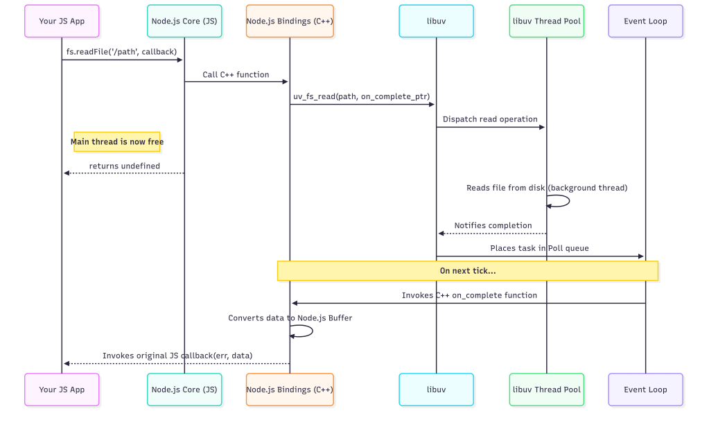
When this line executes, the call first enters the JavaScript part of Node.js’s core fs module. Here, some basic validation happens, like checking that you provided a path and a callback function. Once validated, the call is ready to cross the bridge. It invokes a function in the C++ bindings layer. This is the first crucial translation step: the JavaScript string '/tmp/license-scan.jpg' is converted into a C-style string, and the JavaScript callback function is packaged into a persistent C++ object that can be called later.

Now in the C++ world, the binding function makes a request to libuv, asking it to read the file. It passes the translated file path and a pointer to a C++ function that libuv should invoke upon completion. At this exact moment, the magic of non-blocking I/O happens. Libuv takes the request and adds it to its queue of I/O tasks, which it will service using its background worker thread pool. The C++ binding function, and by extension, the entire fs.readFile call, immediately returns undefined. Your JavaScript code continues executing, completely unblocked. The main thread is now free to handle other requests, like processing another user’s rental booking.

Sometime later, a worker thread from libuv’s pool finishes reading the entire file into a raw memory buffer. It notifies the main event loop that the task is complete. During the event loop’s poll phase, it sees this completed task. This triggers the second half of the journey: the return trip. The event loop invokes the C++ completion function that was passed to libuv earlier. This C++ function takes the raw memory buffer and carefully wraps it in a Node.js Buffer object, which is a data structure V8 can understand. It then prepares to call the original JavaScript callback, passing the Buffer as the data argument (or an Error object if something went wrong).

Finally, the journey ends as the C++ layer invokes your original JavaScript callback function. The data parameter now holds the Buffer containing the image file, and your code can proceed to process it. The entire round-trip, from JavaScript to C++, to libuv’s worker threads, and all the way back, has happened transparently, without ever blocking the main event loop. This elegant, multi-layered architecture is the fundamental reason Node.js can handle immense I/O-bound workloads with such efficiency.

From Knowledge to Mastery

Our journey beyond console.log has taken us deep into the heart of Node.js. We’ve seen that it’s not a single entity, but a powerful trio of components working in perfect harmony. The V8 engine acts as the brilliant, high-speed mind, executing our JavaScript with incredible efficiency. Libuv serves as the tireless workhorse, managing an army of background threads to handle I/O without ever blocking the main stage. And the C++ bindings act as the essential nervous system, seamlessly translating messages between these two worlds. Together, they form a sophisticated system meticulously engineered for one primary goal: building scalable, high-throughput applications that excel at non-blocking I/O.

This knowledge is more than just academic; it’s a toolkit for writing better code. Because you now understand hidden classes and inline caching, you can structure your objects to help V8 generate faster, more optimized code. Because you can visualize the event loop phases, you can finally debug with confidence why your setTimeout seems to fire later than expected or why process.nextTick executes before setImmediate. And because you’ve traced the journey of an I/O call, you have a deep appreciation for why CPU-intensive tasks must be kept off the main thread to keep your application responsive and fast.

But don’t just take my word for it. The true path from knowledge to mastery is through experimentation. We encourage you to roll up your sleeves and see these internals in action. Fire up a Node.js process with the --trace-opt and --trace-deopt flags to watch V8’s JIT compiler work its magic in real-time. Dive into the built-in perf_hooks module to precisely measure the performance of your functions. For a powerful visual perspective, generate a flame graph of your application to see exactly where it’s spending its time. By actively exploring these layers, you will transform your understanding of Node.js and unlock a new level of development expertise.

The Scheduler, The Fiber, and The Reconciler: A Deep Dive into React’s Core


Most React developers are familiar with the concept of the Virtual DOM. We’re taught that when we call setState, React creates a new virtual tree, “diffs” it with the old one, and efficiently updates the actual browser DOM. While true, this high-level explanation barely scratches the surface of the sophisticated engine running under the hood. It doesn’t answer the critical questions: How does React handle multiple, competing updates? What allows it to render fluid animations while also fetching data or responding to user input without freezing the page? The simple diffing algorithm is only the beginning of the story.


The Evolution of React’s Reconciler

Introduction to Reconciliation

At the heart of every React application lies a powerful process known as reconciliation. This is the fundamental mechanism React uses to ensure that the user interface (UI) you see in the browser is always a precise reflection of the application’s current state. Whenever the state of your application changes—perhaps a user clicks a button, data arrives from a server, or an input field is updated—React initiates this reconciliation process to efficiently update the UI.

To understand how this works, we first need to grasp the concept of the Virtual DOM. Instead of directly manipulating the browser’s Document Object Model (DOM), which can be slow and resource-intensive, React maintains a lightweight, in-memory representation of it. This Virtual DOM is essentially a JavaScript object that mirrors the structure of the real DOM. Working with this JavaScript object is significantly faster than interacting with the actual browser DOM.

When a React component renders for the first time, React creates a complete Virtual DOM tree for that component and its children. Let’s consider a simple car rental application. We might have a CarListComponent that displays a list of available vehicles.

import React from 'react';

function CarListComponent({ cars }) {
return (
<div>
<h1>Available Cars</h1>
{cars.map(car => (
<div key={car.id} className="car-item">
<h2>{car.make} {car.model}</h2>
<p>Price per day: ${car.price}</p>
</div>
))}
</div>
);
}

When this component first renders, React builds a Virtual DOM tree that looks something like this (in a simplified view):

{
type: 'div',
props: {
children: [
{ type: 'h1', props: { children: 'Available Cars' } },
// ... and so on for each car
]
}
}

This entire structure exists only in JavaScript memory. React then takes this Virtual DOM and uses it to create the actual DOM elements that are displayed on the screen.

The magic happens when the state changes. Imagine the user applies a filter to see only sedans. This action updates the cars prop, triggering a re-render of CarListComponent. Now, React doesn’t just throw away the old UI and build a new one from scratch. Instead, it creates a new Virtual DOM tree based on the updated state.

With two versions of the Virtual DOM in memory—the previous one and the new one—React performs what is known as a “diffing” algorithm. It efficiently compares, or “diffs,” the new Virtual DOM against the old one to identify the exact, minimal set of changes required to bring the real DOM to the desired state. It walks through both trees, node by node, and compiles a list of mutations. For instance, it might determine that three div elements representing SUVs need to be removed and two new div elements for sedans need to be added.

Once this “diff” is calculated, React proceeds to the final step: it takes this list of changes and applies them to the real browser DOM in a single, optimised batch. This targeted approach is what makes React so performant. By limiting direct manipulation of the DOM to only what is absolutely necessary, it avoids costly reflows and repaints, resulting in a smooth and responsive user experience. This entire cycle—creating a new Virtual DOM on state change, diffing it with the old one, and updating the real DOM—is the essence of reconciliation.

The Stack Reconciler (Pre-Fiber)

Before the release of React 16, the engine driving the reconciliation process was what we now refer to as the Stack Reconciler. Its name comes from its reliance on the call stack to manage the rendering work. This version of the reconciler operated in a synchronous and recursive manner. When a state or prop update occurred, React would start at the root of the affected component tree and recursively traverse the entire structure, calculating the differences and applying them to the DOM.

The key characteristic of this approach was its uninterruptible nature. Once the reconciliation process began, it would continue until the entire component tree was processed and the call stack was empty. This all-or-nothing approach worked well for smaller applications, but its limitations became apparent as user interfaces grew in complexity.

Let’s return to our car rental application to see this in action. Imagine a more complex UI where users can not only see a list of cars but also apply multiple filters, sort the results, and view detailed specifications for each vehicle, all within a single, intricate component tree.

// A hypothetical complex component structure
function CarDashboard({ filters, sortBy }) {
const filteredCars = applyFilters(CARS_DATA, filters);
const sortedCars = applySorting(filteredCars, sortBy);

return (
<div>
<FilterControls />
<SortOptions />
<div className="car-grid">
{sortedCars.map(car => (
<CarCard key={car.id} car={car}>
<CarImage image={car.imageUrl} />
<CarSpecs specs={car.specifications} />
<BookingButton price={car.price} />
</CarCard>
))}
</div>
</div>
);
}

In this example, a single update to the filters prop of CarDashboard would trigger the Stack Reconciler. React would recursively call the render method (or functional component equivalent) for CarDashboard, then for every CarCard, and for every CarImage, CarSpecs, and BookingButton within them. This creates a deep call stack of functions that need to be executed.

The critical issue here is that all of this work happens synchronously on the main thread. The main thread is the single thread in a browser responsible for handling everything from executing JavaScript to responding to user input like clicks and scrolls, and performing layout and paint operations.

If our CarDashboard renders hundreds of cars with deeply nested components, the reconciliation process could take a significant amount of time—perhaps several hundred milliseconds. During this entire period, the main thread is completely blocked. It cannot do anything else. If a user tries to click a button or scroll the page while the Stack Reconciler is busy, the browser won’t be able to respond until the reconciliation is complete. This leads to a frozen or “janky” user interface, creating a poor user experience.

Consider an animation, like a loading spinner, that should be running while the new car list is being prepared. With the Stack Reconciler blocking the main thread, the JavaScript needed to update the animation’s frames cannot run. The result is a stuttering or completely frozen animation. This fundamental limitation—its inability to pause, defer, or break up the rendering work—was the primary motivation for the React team to completely rewrite the reconciler. It became clear that for modern, highly interactive applications, a new approach was needed that could yield to the browser and prioritize work more intelligently.

The Advent of the Fiber Reconciler

To overcome the inherent limitations of the synchronous Stack Reconciler, the React team embarked on a multi-year project to completely rewrite its core algorithm. The result, unveiled in React 16, is the Fiber Reconciler. This wasn’t just an update; it was a fundamental rethinking of how reconciliation should work, designed specifically for the complex and dynamic user interfaces of modern web applications.

The primary goal of the Fiber Reconciler is to enable incremental and asynchronous rendering. Unlike its predecessor, Fiber is designed to be interruptible. It can break down the rendering work into smaller, manageable chunks, and pause its work to yield control back to the browser’s main thread. This means that high-priority updates, like user input or critical animations, can be handled immediately, without having to wait for a large, time-consuming render to complete.

At its core, Fiber introduces a new data structure, also called a “fiber,” which represents a unit of work. Instead of a recursive traversal that fills the call stack, React now creates a linked list of these fiber objects. This new architecture allows React to walk through the component tree, process a few units of work, and then, if a higher-priority task appears or if it’s running out of its allotted time slice, it can pause the reconciliation process. Once the main thread is free again, React can pick up right where it left off.

Let’s revisit our complex car rental application to see the profound impact of this change.

// The same complex component from the previous section
function CarDashboard({ filters, sortBy }) {
// ... filtering and sorting logic ...

// A new component to show a typing indicator
const [isTyping, setIsTyping] = useState(false);

return (
<div>
<FilterControls onTypingChange={setIsTyping} />
<SortOptions />
{isTyping && <div className="typing-indicator">Filtering...</div>}
<div className="car-grid">
{/* ... mapping over sortedCars ... */}
</div>
</div>
);
}

Imagine a user is typing in a search box within the <FilterControls /> component. With the old Stack Reconciler, each keystroke would trigger a full, synchronous re-render of the entire car-grid. If rendering the grid takes 200ms, but the user is typing a new character every 100ms, the UI would feel sluggish and unresponsive. The typing-indicator might never even appear because the main thread would be perpetually blocked by the rendering work.

With the Fiber Reconciler, the outcome is dramatically different. As the user types, React begins the rendering work for the updated car-grid. However, it doesn’t do it all at once. It processes a few CarCard components, then yields to the main thread. This gives the browser a chance to process the next keystroke or render the typing-indicator. The reconciliation of the car-grid happens incrementally, in the background, without freezing the UI.

This ability to pause, resume, and prioritize work is the superpower of the Fiber Reconciler. It allows React to build fluid and responsive user experiences, even in applications with complex animations, demanding data visualizations, and intricate component hierarchies. It lays the groundwork for advanced features like Concurrent Mode, Suspense for data fetching, and improved server-side rendering, fundamentally changing what’s possible in a React application.

Deconstructing the Fiber Architecture

What is a Fiber?

At the heart of React’s modern reconciler is a plain JavaScript object called a fiber. It’s much more than just a data structure; a fiber represents a unit of work. Instead of thinking of rendering as a single, monolithic task, the Fiber architecture breaks down the rendering of a component tree into thousands of these discrete units. This allows React to start, pause, and resume rendering work, which is the key to enabling non-blocking, asynchronous rendering.

Every single component instance in your application, whether it’s a class component, a function component, or even a simple HTML tag like div, has a corresponding fiber object. Let’s examine the essential properties of a fiber object to understand how it orchestrates the rendering process, using our car rental application as a backdrop.

Imagine we have a CarCard component that receives new props. React will create a fiber object for it. While the actual fiber has many properties, we’ll focus on the most critical ones.

// A simplified representation of a CarCard component
function CarCard({ car }) {
return (
<div key={car.id} className="card">
<h3>{car.make} {car.model}</h3>
<p>Price: ${car.price}</p>
</div>
);
}

A fiber for this component would contain the following key properties:

  • type and key: These properties identify the component associated with the fiber. The type would point to the CarCard function itself. The key (in our case, car.id) is the unique identifier you provide in a list, which helps React efficiently track additions, removals, and re-orderings without having to re-render every item.
  • child, sibling and return pointers: This is where Fiber departs dramatically from the old Stack Reconciler. Instead of relying on recursive function calls to traverse the component tree, a fiber tree is a linked list. Each fiber has pointers to its first child, its next sibling, and its return (or parent) fiber. This flat, pointer-based structure allows React to traverse the tree without deep recursion, meaning it can stop at any point and know exactly how to resume later.
  • pendingProps and memoizedProps: These properties are crucial for determining if a component needs to re-render. memoizedProps holds the props that were used to render the component last time. pendingProps holds the new props that have just been passed down from the parent. During the reconciliation process, React compares pendingProps with memoizedProps. If they are different, the component needs to be updated. For our CarCard, if the car.price in pendingProps is different from the price in memoizedProps, React knows it must re-render this component.
  • alternate: This property is the linchpin of Fiber’s ability to perform work without affecting the visible UI. It implements a technique called double buffering. At any given time, there are two fiber trees: the current tree, which represents the UI currently on the screen, and the work-in-progress tree, which is where React builds updates off-screen. The alternate property of a fiber in the current tree points to its corresponding fiber in the work-in-progress tree, and vice-versa. When a state update occurs, React clones the affected fibers from the current tree to create the work-in-progress tree. All the diffing and rendering work happens on this off-screen tree. Once the work is complete, React atomically swaps the work-in-progress tree to become the new current tree. This process is seamless and prevents UI tearing or showing inconsistent states to the user.

By representing the entire application as a tree of these granular fiber objects, React gains incredible control over the rendering process. It’s no longer a black box that runs to completion. Instead, it’s a series of schedulable units of work that can be executed according to their priority, ensuring that the most critical updates are always handled first, leading to a fluid and responsive application.

How Fiber Enables Asynchronous Rendering

The true power of the Fiber architecture lies in how it uses the linked-list structure of the fiber tree to achieve asynchronous rendering. Because each fiber is a distinct unit of work with explicit pointers to its child, sibling, and return fibers, React is no longer forced into an uninterruptible, recursive traversal. Instead, it can walk the tree incrementally and, most importantly, pause at any time without losing its place.

This process is managed by a work loop. When a render is triggered, React starts at the root of the work-in-progress tree and begins traversing it according to a specific algorithm:

  1. Begin Work: React performs the work for the current fiber. This involves comparing its pendingProps to its memoizedProps to see if it needs to update.
  2. Move to Child: If the fiber has a child, React makes that child the next unit of work.
  3. Move to Sibling: If the fiber has no child, React moves to its sibling and makes that the next unit of work.
  4. Return: If the fiber has no child and no sibling, React moves up the tree using the return pointer until it finds a fiber with a sibling to work on, or until it completes the entire tree.

This predictable, manual traversal is the key. Between processing any two fibers, React can check if there’s more urgent work to do, such as responding to user input. If there is, it can simply pause the work loop, leaving the fiber tree in its current state, and yield to the main thread.

Let’s visualize this with our car rental application. Assume we have a list of 100 CarCard components to render after a filter is applied.

// A parent component that renders a list of CarCards
function CarList({ cars }) {
// A high-priority state update for user input
const [inputValue, setInputValue] = useState('');

return (
<div>
<input
value={inputValue}
onChange={e => setInputValue(e.target.value)}
placeholder="Type to highlight a car..."
/>
<div className="grid">
{cars.map(car => <CarCard key={car.id} car={car} />)}
</div>
</div>
);
}

When the cars prop changes, React starts its work loop on the <div className=”grid”>. It processes the first CarCard fiber, then its sibling (the second CarCard), and so on. Now, imagine after processing the tenth CarCard, the user starts typing into the <input>.

The onChange event is a high-priority update. The Fiber reconciler, after completing work on the tenth CarCard, can detect this pending high-priority update. Instead of continuing to the eleventh CarCard, it pauses the low-priority rendering of the list. It records its progress—knowing the next unit of work is the eleventh CarCard—and yields control to the main thread.

The browser is now free to handle the input event, updating the inputValue state and re-rendering the input field. The user sees immediate feedback for their typing, and the UI remains fluid. Once the main thread is idle again, React resumes its previous work exactly where it left off, beginning its work loop on the eleventh CarCard fiber. This ability to pause, yield, and resume—or even abort the old work if new props come in—is what we call asynchronous rendering. It ensures that long rendering tasks don’t block the main thread, leading to a vastly superior and more responsive user experience.

The Role of the Scheduler

Prioritizing Updates

While the Fiber Reconciler provides the mechanism for pausing and resuming work, it doesn’t decide when that should happen. That crucial responsibility falls to another key part of React’s core: the Scheduler. The Scheduler acts as a sophisticated traffic controller for all pending state updates, organizing them into a prioritized queue. Its fundamental job is to tell the Reconciler which unit of work to perform next, ensuring that the most critical updates are processed first, leading to a fluid and responsive application.

To achieve this, the Scheduler assigns a priority level to every update. This allows React to differentiate between an urgent user interaction and a less critical background task. Let’s explore these priority levels within the context of our car rental application.

The highest priority is Synchronous. This level is reserved for updates that must be handled immediately and cannot be deferred. A primary example is updates to uncontrolled inputs. If a user is typing into a search box, they expect to see their characters appear instantly. React handles these updates synchronously to guarantee immediate feedback, as any delay would feel broken.

Next is what can be considered Task or User-Blocking priority. These are high-priority updates, typically initiated by direct user interaction, that should be completed quickly to avoid making the UI feel sluggish. For instance, when a user clicks a button to apply a “SUV” filter, they expect the list of cars to update promptly.

import { useState } from 'react';

function FilterComponent({ onFilterChange }) {
const handleFilterClick = () => {
// This setState call is treated as a high-priority, user-blocking update.
// The user has clicked something and expects a fast response.
onFilterChange('SUV');
};

return <button onClick={handleFilterClick}>Show SUVs</button>;
}

In this case, the Scheduler ensures that the work to re-render the car list begins almost immediately. It’s not strictly synchronous—it can still be broken up by the Fiber Reconciler—but it’s placed at the front of the queue, ahead of any lower-priority work.

A distinct level exists for Animation priority. This is for updates that need to complete within a single animation frame to create smooth visual effects, such as those managed by requestAnimationFrame. Imagine in our car rental app, clicking on a car card smoothly expands it to reveal more details. The state update that controls this expansion—for example, changing its height from 100px to 400px—would be scheduled with animation priority to prevent visual stuttering or “jank.”

Finally, there is Idle priority. This is the lowest priority level, reserved for background tasks or deferred work that can be performed whenever the browser is idle. This is perfect for non-essential tasks that don’t impact the current user experience. For example, we could pre-fetch data for a “You Might Also Like” section while the user is browsing the main car list.

import { useEffect } from 'react';

// A custom hook to pre-fetch data when the browser is idle
function useIdlePrefetch(url) {
useEffect(() => {
// The 'startTransition' API (or a similar internal mechanism)
// tells React to treat this state update as low-priority.
React.startTransition(() => {
// This fetch call and subsequent state update will only run
// when the main thread is not busy with higher-priority tasks.
fetch(url).then(res => res.json()).then(setData);
});
}, [url]);
}

By intelligently categorizing every update, the Scheduler provides the Reconciler with a clear order of operations. It ensures that a user’s click is always more important than a background data fetch, and that a smooth animation is never interrupted by a slow re-render, forming the foundation of a truly performant and user-centric application.

Yielding to the Main Thread

The Scheduler’s ability to prioritize updates would be of little use without a mechanism to act on those priorities. This is where the concept of yielding to the main thread becomes critical. The browser’s main thread is a single, precious resource responsible for executing JavaScript, handling user interactions, and painting pixels to the screen. If a single task, like rendering a large component tree, monopolizes this thread for too long, the entire application freezes. This is what users perceive as “jank” or unresponsiveness.

To prevent this, the Scheduler and the Fiber Reconciler work in close cooperation. The Scheduler doesn’t just tell the Reconciler what to do next; it also gives it a deadline. It essentially says, “Work on this task, but you must yield control back to me if a higher-priority task arrives or if you’ve been working for more than a few milliseconds (a time slice).” This cooperative scheduling ensures that no single rendering task can ever block the main thread for a significant period.

Let’s see how this plays out in our car rental application. Imagine we have a feature that renders a complex, data-heavy AnalyticsDashboard component. This is a low-priority update that we trigger in the background. At the same time, the user can click a “Quick Book” button for a featured car, which is a high-priority action.

function CarRentalApp() {
const [showDashboard, setShowDashboard] = useState(false);

// High-priority action: A user clicks to book a car
const handleQuickBook = () => {
// This is a high-priority update
alert('Car booked! Confirmation will be sent shortly.');
};

useEffect(() => {
// Low-priority action: We decide to render a heavy component
// in the background after the initial page load.
// React's 'startTransition' marks this as a non-urgent update.
React.startTransition(() => {
setShowDashboard(true);
});
}, []);

return (
<div>
<h1>Featured Car</h1>
<button onClick={handleQuickBook}>Quick Book Now</button>
<hr />
{/* The AnalyticsDashboard is a very large and slow component */}
{showDashboard && <AnalyticsDashboard />}
</div>
);
}

Here’s the sequence of events:

  1. Low-Priority Work Begins: After the initial render, the useEffect hook fires. The startTransition call tells the Scheduler that setting showDashboard to true is a low-priority update. The Scheduler instructs the Reconciler to start rendering the AnalyticsDashboard.
  2. Work in Progress: The Reconciler begins its work loop, processing the fibers for the AnalyticsDashboard one by one. This is a slow component, and the work will take, say, 300 milliseconds to complete.
  3. High-Priority Interruption: After 50 milliseconds of rendering the dashboard, the user clicks the “Quick Book Now” button. This onClick event is a high-priority task.
  4. The Scheduler Intervenes: The Scheduler immediately sees this new, high-priority update. It checks its clock and sees that the Reconciler has been working on the low-priority task. It signals to the Reconciler that it must yield.
  5. Reconciler Pauses: After finishing its current unit of work (the fiber it’s currently processing), the Reconciler pauses. It doesn’t throw away its progress on the AnalyticsDashboard; it simply leaves the work-in-progress tree in its partially completed state.
  6. Main Thread is Free: Control is returned to the main thread. The browser is now free to execute the handleQuickBook event handler. The alert appears instantly. The user gets immediate feedback.
  7. Work Resumes: Once the high-priority task is complete and the main thread is idle, the Scheduler tells the Reconciler it can resume its work on the AnalyticsDashboard right where it left off.

This act of yielding is the cornerstone of a responsive React application. It ensures that no matter how much work is happening in the background, the application is always ready to respond to the user’s most recent and important interactions.

The Two Phases of Rendering

The Render Phase (or “Reconciliation Phase”)

The first stage of React’s update process is the Render Phase. During this phase, React discovers what changes need to be made to the UI. Its goal is to create a new “work-in-progress” Fiber tree that represents the future state of your application. It’s crucial to understand that this phase is purely computational; it involves calling your components and comparing the results with the previous render, but it does not touch the actual browser DOM.

The most important characteristic of the Render Phase is that it is asynchronous and interruptible. Because React is only working with its internal fiber objects, it can perform this work in small chunks, pausing to yield to the main thread for more urgent tasks, or even discarding the work altogether if a newer, higher-priority update comes in. This is the magic that prevents UI blocking.

Several component lifecycle methods are executed during this phase. This is the point where React gives you, the developer, an opportunity to influence the rendering outcome. These methods include the constructor, getDerivedStateFromProps, shouldComponentUpdate, and, most famously, the render method itself.

Let’s consider a CarDetails class component in our application that displays information about a selected vehicle.

class CarDetails extends React.Component {
constructor(props) {
super(props);
// 1. constructor: Runs once. Good for initializing state.
this.state = { isFavorite: false };
}

static getDerivedStateFromProps(nextProps, prevState) {
// 2. getDerivedStateFromProps: Runs on every render.
// Use this to derive state from props over time.
// For example, resetting a view when the car ID changes.
return null; // Or return an object to update state
}

shouldComponentUpdate(nextProps, nextState) {
// 3. shouldComponentUpdate: Your chance to optimize.
// If the price hasn't changed, we can skip this entire update.
if (this.props.car.price === nextProps.car.price) {
return false; // Tells React to bail out of the render process for this component
}
return true;
}

render() {
// 4. render: The core of the phase. Purely describes what the UI should look like.
const { car } = this.props;
return (
<div>
<h1>{car.make} {car.model}</h1>
<p>Price: ${car.price}</p>
{/* ... other details ... */}
</div>
);
}
}

In older versions of React, this phase also included methods like componentWillMount, componentWillReceiveProps, and componentWillUpdate. These are now prefixed with UNSAFE_ because the interruptible nature of the Render Phase makes them dangerous for certain tasks, particularly side effects like making API calls.

Why are they considered unsafe? Imagine our application starts rendering an update to the CarDetails component because a new discount is being calculated. React calls UNSAFE_componentWillUpdate. Inside this method, we might have naively placed an API call to log this “view update” event.

// UNSAFE_componentWillUpdate(nextProps) {
// // DANGEROUS: This side effect is in the Render Phase.
// api.logEvent('user is viewing updated price', nextProps.car.id);
// }

Now, before this low-priority render can complete, the user clicks a button for a high-priority action. The Scheduler interrupts the CarDetails render, discards the work, and handles the user’s click. Later, React restarts the CarDetails render from scratch, and UNSAFE_componentWillUpdate is called a second time for the same logical update. Our logging service would now have two duplicate events. Worse, the first render could have been aborted entirely, meaning the method was called but the UI was never actually updated, leading to inconsistent analytics.

Because the Render Phase can be paused, restarted, or aborted, any code within it may be executed multiple times or not at all before a final decision is made. Therefore, this phase must be kept “pure”—free of side effects. Its sole responsibility is to describe the desired UI, leaving all mutations and side effects to the next, non-interruptible phase.

The Commit Phase

The Commit Phase is the second and final stage of React’s rendering process. This is where React takes the “work-in-progress” Fiber tree, which was calculated during the Render Phase, and applies the necessary changes to the actual browser DOM. Once this phase begins, it is synchronous and cannot be interrupted. This uninterruptible nature is crucial because it guarantees that the DOM is updated in a single, consistent batch, preventing users from ever seeing a partially updated or broken UI.

Because the Commit Phase runs only after a render has been finalized and is guaranteed to complete, it is the safe and correct place to run side effects. This includes tasks like making API calls, setting up subscriptions, or manually manipulating the DOM. The lifecycle methods that execute during this phase are specifically designed for these kinds of interactions.

Let’s explore these lifecycle methods using a CarBookingWidget component, which might need to interact with the DOM and fetch data after it renders.

class CarBookingWidget extends React.Component {
chatRef = React.createRef();

// 1. getSnapshotBeforeUpdate: Runs right before the DOM is updated.
// Its return value is passed to componentDidUpdate.
getSnapshotBeforeUpdate(prevProps, prevState) {
// Let's capture the scroll position of a chat log before a new message is added.
if (prevProps.messages.length < this.props.messages.length) {
const chatLog = this.chatRef.current;
return chatLog.scrollHeight - chatLog.scrollTop;
}
return null;
}

// 2. componentDidUpdate: Runs immediately after the update is committed to the DOM.
// Perfect for side effects that depend on the new props or the DOM being updated.
componentDidUpdate(prevProps, prevState, snapshot) {
// If we have a snapshot, we can use it to maintain the scroll position.
if (snapshot !== null) {
const chatLog = this.chatRef.current;
chatLog.scrollTop = chatLog.scrollHeight - snapshot;
}

// A common use case: Fetch new data when a prop like an ID changes.
if (this.props.carID !== prevProps.carID) {
fetch(`/api/cars/${this.props.carID}/addons`).then(/* ... */);
}
}

// 3. componentDidMount: Runs once, after the component is first mounted to the DOM.
// The ideal place for initial data loads and setting up subscriptions.
componentDidMount() {
// Example: Connect to a WebSocket for real-time price updates for this car.
this.subscription = setupPriceListener(this.props.carID, (newPrice) => {
this.setState({ price: newPrice });
});
}

// 4. componentWillUnmount: Runs right before the component is removed from the DOM.
// Essential for cleanup to prevent memory leaks.
componentWillUnmount() {
// Clean up the subscription when the widget is no longer needed.
this.subscription.unsubscribe();
}

render() {
// ... JSX for the booking widget ...
return <div ref={this.chatRef}>{/* ... messages ... */}</div>;
}
}

In this phase, you can be confident that the UI is in a consistent state. componentDidMount and componentDidUpdate are invoked after the DOM has been updated, so any DOM measurements you take will reflect the final layout. getSnapshotBeforeUpdate provides a unique window to capture information from the DOM before it changes. Finally, componentWillUnmount provides a critical hook to clean up any long-running processes when the component is destroyed. By strictly separating the pure calculations of the Render Phase from the side effects of the Commit Phase, React provides a powerful, predictable, and safe model for building complex applications.

Bringing It All Together

Our deep dive has taken us on a journey from the early days of React’s synchronous Stack Reconciler to the sophisticated, modern engine that powers today’s applications. We’ve seen how the limitations of an uninterruptible, recursive rendering process led to the creation of a groundbreaking new system. This system is built on the elegant interplay of three core components: the Fiber Reconciler, the Scheduler, and a distinct two-phase rendering process. Together, they form the foundation that makes React a powerful tool for building complex, high-performance user interfaces.

We’ve deconstructed the Fiber architecture, understanding that each “fiber” is not just a node in a tree, but a schedulable unit of work. Its pointer-based, linked-list structure is the key that unlocks the ability to pause, resume, or even abort rendering work without losing context. We then introduced the Scheduler, the intelligent traffic controller that prioritizes every update, ensuring that a user’s click is always handled before a background data fetch. Finally, we saw how this all comes together in the two-phase rendering model. The interruptible Render Phase safely calculates what needs to change without touching the DOM, while the synchronous Commit Phase applies those changes in one swift, consistent batch.

This advanced architecture is precisely why React can handle fluid animations, complex user interactions, and large-scale data updates without freezing the browser. It is the reason developers can build applications that feel fast and responsive, even when immense computational work is happening behind the scenes.

Understanding these internal mechanisms is more than just an academic exercise; it directly influences how we write better React code. Knowing that the Render Phase can be interrupted reinforces the critical importance of keeping our render methods and functional components pure and free of side effects. Recognizing that the Commit Phase is the safe place for mutations encourages the correct use of lifecycle methods and hooks like useEffect for API calls and subscriptions. When you use modern APIs like startTransition to wrap a non-urgent state update, you are directly tapping into the power of the Scheduler, telling it to treat that work as deferrable.

By grasping the “why” behind React’s architecture, we move beyond simply following patterns and begin to make informed decisions. We write more resilient, efficient, and performant code because we understand the elegant and powerful dance happening inside React every time our application’s state changes.

Too many llamas? Running AI locally


In the rapidly evolving landscape of artificial intelligence, understanding the distinctions between various tools and models is crucial for developers and researchers. This blog post aims to elucidate the differences between the LLaMA model, llama.cpp, and Ollama. While the LLaMA model serves as the foundational large language model developed by Meta, llama.cpp is an open-source C++ implementation designed to run LLaMA efficiently on local hardware. Building upon llama.cpp, Ollama offers a user-friendly interface with additional optimizations and features. By exploring these distinctions, readers will gain insights into selecting the appropriate tool for their AI applications.


What is the LLaMA Model?

LLaMA (Large Language Model Meta AI) is a series of open-weight large language models (LLMs) developed by Meta (formerly Facebook AI). Unlike proprietary models like GPT-4, LLaMA models are released under a research-friendly license, allowing developers and researchers to experiment with state-of-the-art AI while maintaining control over data and privacy.

LLaMA models are designed to be smaller and more efficient than competing models while maintaining strong performance in natural language understanding, text generation, and reasoning.

LLaMA is a Transformer-based AI model that processes and generates human-like text. It is similar to OpenAI’s GPT models but optimized for efficiency. Meta’s goal with LLaMA is to provide smaller yet powerful language models that can run on consumer hardware.

Unlike GPT-4, which is closed-source, LLaMA models are available to researchers and developers, enabling:

  • Customisation & fine-tuning for specific applications
  • Running models locally instead of relying on cloud APIs
  • Improved privacy since queries don’t need to be sent to external servers

LLaMA models are powerful, but they are not the only open-source LLMs available. Let’s compare them with other major models:

FeatureLLaMA 2GPT-4 (OpenAI)Mistral 7BMixtral (MoE)
Size7B, 13B, 70BProprietary7B12.9B (MoE)
Open-Source?✅ Yes❌ No✅ Yes✅ Yes
PerformanceGPT-3.5 Level🔥 BestBetter than LLaMA 2-7BOutperforms LLaMA 2-13B
Fine-Tunable?✅ Yes❌ No✅ Yes✅ Yes
Runs on CPU?✅ Yes (with llama.cpp)❌ No✅ Yes❌ Requires GPU
Best ForChatbots, research, AI appsGeneral AI, commercial APIsFast reasoning, efficiencyScalable AI applications

LLaMA models are versatile and can be used for various applications:

  • AI Chatbots
  • Code Generation
  • Scientific Research
  • Private AI Applications

LLaMA is one of the most influential open-weight LLMs, offering a balance between power, efficiency, and accessibility. Unlike closed-source models like GPT-4, LLaMA allows developers to run AI locally, fine-tune models, and ensure data privacy.

AI Model Quantisation: Making AI Models Smaller and Faster

AI models, especially deep learning models like large language models (LLMs) and speech recognition systems, are huge. They require massive amounts of computational power and memory to run efficiently. This is where model quantisation comes in—a technique that reduces the size of AI models and speeds up inference while keeping accuracy as high as possible.

Quantisation is the process of converting a model’s parameters (weights and activations) from high-precision floating-point numbers (e.g., 32-bit float, FP32) into lower-precision numbers (e.g., 8-bit integer, INT8). This reduces the memory footprint and improves computational efficiency, allowing AI models to run on less powerful hardware like CPUs, edge devices, and mobile phones.

When an AI model is trained, it typically uses 32-bit floating-point (FP32) numbers to represent its weights and activations. These provide high precision but require a lot of memory and processing power. Quantisation converts these high-precision numbers into lower-bit representations, such as:

  • FP32 → FP16 (Half-precision floating-point)
  • FP32 → INT8 (8-bit integer)
  • FP32 → INT4 / INT2 (Ultra-low precision)

The lower the bit-width, the smaller and faster the model becomes, but at the cost of some accuracy. Assume we have a weight value stored as a 32-bit float:

Weight (FP32) = 0.87654321

If we convert this to 8-bit integer (INT8):

Weight (INT8) ≈ 87 (scaled down)

Even though we lose some precision, the model remains usable while consuming much less memory and processing power.

There are several types of quantisation:

  • Post-Training Quantisation – PTQ (Applied after training, converts model weights and activations to lower precision, faster but may cause some accuracy loss)
  • Quantisation-Aware Training – QAT (The model is trained while simulating lower precision, maintains higher accuracy compared to PTQ, more computationally expensive during training, used when accuracy is critical e.g., in medical AI models)
  • Dynamic Quantisation (Only weights are quantised; activations remain in higher precision, applied at runtime, making it more flexible, used in NLP models like llama.cpp for efficient inference)
  • Weight-Only Quantisation (Only model weights are quantised, not activations, used in GGUF/GGML models to run LLMs efficiently on CPUs)

Some of the benefits of quantisation are:

  • Reduces Model Size – Helps fit large AI models on small devices.
  • Speeds Up Inference – Allows faster processing on CPUs and edge devices.
  • Lower Power Consumption – Essential for mobile and embedded applications.
  • Enables AI on Consumer Hardware – Allows running LLMs (like llama.cpp) on laptops and smartphones.

Real world examples of quantisation include:

  • Whisper.cpp – Uses INT8 quantisation for speech-to-text transcription on CPUs.
  • Llama.cpp – Uses GGUF/GGML quantisation to run LLaMA models efficiently on local machines.
  • TensorFlow Lite & ONNX – Deploy AI models on mobile and IoT devices using quantized versions.

Quantisation is one of the most effective techniques for optimising AI models, making them smaller, faster, and more efficient. It allows complex deep learning models to run on consumer-grade hardware without sacrificing too much accuracy. Whether you’re working with text generation, speech recognition, or computer vision, quantisation is a game-changer in bringing AI to the real world.

Model fine-tuning with LoRA

Low-Rank Adaptation (LoRA) is a technique introduced to efficiently fine-tune large-scale pre-trained models, such as Large Language Models (LLMs), for specific tasks without updating all of their parameters. As models grow in size, full fine-tuning becomes computationally expensive and resource-intensive. LoRA addresses this challenge by freezing the original model’s weights and injecting trainable low-rank matrices into each layer of the Transformer architecture. This approach significantly reduces the number of trainable parameters and the required GPU memory, making the fine-tuning process more efficient.  

In traditional fine-tuning, all parameters of a pre-trained model are updated, which is not feasible for models with billions of parameters. LoRA proposes that the changes in weights during adaptation can be approximated by low-rank matrices. By decomposing these weight updates into the product of two smaller matrices, LoRA introduces additional trainable parameters that are much fewer in number. These low-rank matrices are integrated into the model’s layers, allowing for task-specific adaptation while keeping the original weights intact.  

LoRA presents several advantages:

  • Parameter Efficiency: LoRA reduces the number of trainable parameters by orders of magnitude. For instance, fine-tuning GPT-3 with LoRA can decrease the trainable parameters by approximately 10,000 times compared to full fine-tuning.  
  • Reduced Memory Footprint: By updating only the low-rank matrices, LoRA lowers the GPU memory requirements during training, making it feasible to fine-tune large models on hardware with limited resources.  
  • Maintained Performance: Despite the reduction in trainable parameters, models fine-tuned with LoRA perform on par with, or even better than, those fine-tuned traditionally across various tasks.  

LoRA has been applied successfully in various domains, including:

  • Natural Language Processing (NLP): Fine-tuning models for specific tasks like sentiment analysis, translation, or question-answering.
  • Computer Vision: Adapting vision transformers to specialised image recognition tasks.
  • Generative Models: Customising models like Stable Diffusion for domain-specific image generation.

By enabling efficient and effective fine-tuning, LoRA facilitates the deployment of large models in specialised applications without the associated computational burdens of full model adaptation.

Using llama.cpp to Run Large Language Models Locally

With the rise of large language models (LLMs) like OpenAI’s GPT-4 and Meta’s LLaMA series, the demand for running these models efficiently on local machines has grown. However, most large-scale AI models require powerful GPUs and cloud-based services, which can be costly and raise privacy concerns.

Enter llama.cpp, a highly optimised C++ implementation of Meta’s LLaMA models that allows users to run language models directly on CPUs. This makes it possible to deploy chatbots, assistants, and other AI applications on personal computers, edge devices, and even mobile phones—without relying on cloud services.

What is llama.cpp?

llama.cpp is an efficient CPU-based inference engine for running Meta’s LLaMA models (LLaMA 1, LLaMA 2, and variants like Mistral, Phi, and Qwen) on Windows, macOS, Linux, and even ARM-based devices. It uses quantisation techniques to reduce the model size and memory requirements, making it possible to run LLMs on consumer-grade hardware.

The key features of llama.cpp are:

  • CPU-based execution – No need for GPUs.
  • Quantisation support – Reduces model size with minimal accuracy loss.
  • Multi-platform – Runs on Windows, Linux, macOS, Raspberry Pi, and Android.
  • Memory efficiency – Optimised for low RAM usage.
  • GGUF format – Uses an efficient binary format for LLaMA models.

Installing llama.cpp

The minimum system requirements for llama.cpp are:

  • OS: Windows, macOS, or Linux.
  • CPU: Intel, AMD, Apple Silicon (M1/M2), or ARM-based processors.
  • RAM: 4GB minimum, 8GB+ recommended for better performance.
  • Dependencies: gcc, make, cmake, python3, pip

To install on Linux/macOS, first clone the repository:

git clone https://github.com/ggerganov/llama.cpp
cd llama.cpp

Then, build the project:

make

This compiles the main executable for CPU inference.

On Windows, install MinGW-w64 or use WSL (Windows Subsystem for Linux). Then, open a terminal (PowerShell or WSL) and run:

git clone https://github.com/ggerganov/llama.cpp
cd llama.cpp
make

Alternatively, you can use Python Bindings. llama.cpp provides Python bindings for easy usage:

pip install llama-cpp-python

Downloading and Preparing Models

Meta’s LLaMA models require approval for access. However, open-weight alternatives like Mistral, Phi, and Qwen can be used freely. To download a model, visit Hugging Face and search for LLaMA 2 GGUF models. Download a quantised model, e.g., llama-2-7b.Q4_K_M.gguf.

If you have raw LLaMA models, you must convert them to the GGUF format. First, install transformers:

pip install transformers

Then, convert:

python convert.py --model /path/to/llama/model

Once you have a GGUF model, you can start chatting!

./main -m models/llama-2-7b.Q4_K_M.gguf -p "Tell me a joke"

This runs inference using the model and generates a response. To run a chatbot session:

./main -m models/llama-2-7b.Q4_K_M.gguf --interactive

It will allow continuous interaction, just like ChatGPT.

If needed, you can quantise a model using one of the available levels:

  • Q8_0 – High accuracy, large size.
  • Q6_K – Balanced performance and accuracy.
  • Q4_K_M – Optimised for speed and memory.
  • Q2_K – Ultra-low memory, reduced accuracy.

You can quantise a model using:

python quantize.py --model llama-2-7b.gguf --type Q4_K_M

This produces a GGUF file that is much smaller and runs faster.

To improve performance, use more CPU threads:

./main -m models/llama-2-7b.Q4_K_M.gguf -t 8

This will use 8 threads for inference.

If you have a GPU, you can enable acceleration:

make LLAMA_CUBLAS=1

This allows CUDA-based inference on NVIDIA GPUs.

Fine-tuning

With the power of llama.cpp and LoRA, you can build advanced chatbots, specialised assistants and domain-specific NLP solutions, all running locally, with full control over data and privacy.

Fine-tuning with llama.cpp requires a dataset in JSONL format (JSON Lines), which is a widely-used structure for text data in machine learning. Each line in the JSONL file represents an input-output pair. This format allows the model to learn a mapping from inputs (prompts) to outputs (desired completions):

{"input": "What is the capital of France?", "output": "Paris"}
{"input": "Translate to French: apple", "output": "pomme"}
{"input": "Explain quantum mechanics.", "output": "Quantum mechanics is a fundamental theory in physics..."}

To create a dataset, collect data relevant to your task. For example:

  • Question-Answer Pairs – For a Q&A bot.
  • Translation Examples – For a language translation model.
  • Dialogue Snippets – For chatbot fine-tuning.

Once you have the JSONL dataset ready, you can fine-tune your llama.cpp model using finetune.py. This script utilizes LoRA (Low-Rank Adaptation) to efficiently train the model.

First, you need to install the required libraries:

pip install torch transformers datasets peft bitsandbytes

You can now run finetune.py using the following command:

python finetune.py --model models/llama-2-7b.Q4_K_M.gguf --data dataset.jsonl --output-dir lora-output

After fine-tuning, the LoRA adapters must be merged with the base model to produce a single, fine-tuned model file.

python merge_lora.py --base models/llama-2-7b.Q4_K_M.gguf --lora lora-output --output models/llama-2-7b-finetuned.gguf

You can test the fine-tuned model using llama.cpp to see how it performs:

./main -m models/llama-2-7b-finetuned.gguf -p "What is the capital of France?"

Interesting Models to Run on llama.cpp

There are several models that you can run on llama.cpp:

1. LLaMA 2

  • Creator: Meta
  • Variants: 7B, 13B, 70B
  • Use Cases: General-purpose chatbot, knowledge retrieval, creative writing
  • Best Quantized Version: Q4_K_M (balanced accuracy and speed)
  • Why It’s Interesting: LLaMA 2 is one of the most powerful open-weight language models, comparable to GPT-3.5 in many tasks. It serves as the baseline for experimentation.

Example Usage in llama.cpp:

./main -m models/llama-2-13b.Q4_K_M.gguf -p "Explain the theory of relativity in simple terms."

2. Mistral 7B

  • Creator: Mistral AI
  • Variants: 7B (densely trained)
  • Use Cases: Chatbot, reasoning, math, structured answers
  • Best Quantized Version: Q6_K
  • Why It’s Interesting: Mistral 7B is optimized for factual accuracy and reasoning. It outperforms LLaMA 2 in some tasks despite being smaller.

Example Usage:

./main -m models/mistral-7b.Q6_K.gguf -p "Summarize the latest advancements in quantum computing."

3. Mixtral (Mixture of Experts)

  • Creator: Mistral AI
  • Variants: 12.9B (only 2 experts active at a time)
  • Use Cases: High-performance chatbot, research assistant
  • Best Quantized Version: Q5_K_M
  • Why It’s Interesting: Unlike standard models, Mixtral is a Mixture of Experts (MoE) model, meaning it activates only two out of eight experts per token. This makes it more efficient than similarly sized dense models.

Example Usage:

./main -m models/mixtral-8x7b.Q5_K_M.gguf --interactive

4. Code LLaMA

  • Creator: Meta
  • Variants: 7B, 13B, 34B
  • Use Cases: Code generation, debugging, explaining code
  • Best Quantized Version: Q4_K
  • Why It’s Interesting: This model is fine-tuned for programming tasks. It can generate Python, JavaScript, C++, Rust, and more.

Example Usage:

./main -m models/code-llama-13b.Q4_K.gguf -p "Write a Python function to reverse a linked list."

5. Phi-2

  • Creator: Microsoft
  • Variants: 2.7B
  • Use Cases: Math, logic, reasoning, lightweight chatbot
  • Best Quantized Version: Q5_K_M
  • Why It’s Interesting: Despite being only 2.7B parameters, Phi-2 is surprisingly strong in logical reasoning and problem-solving, outperforming models twice its size.

Example Usage:

./main -m models/phi-2.Q5_K_M.gguf -p "Solve the equation: 5x + 7 = 2x + 20."

6. Qwen-7B

  • Creator: Alibaba
  • Variants: 7B, 14B
  • Use Cases: Conversational AI, structured text generation
  • Best Quantized Version: Q4_K_M
  • Why It’s Interesting: Qwen models are multilingual and trained with high-quality data, making them excellent for chatbots.

Example Usage:

./main -m models/qwen-7b.Q4_K_M.gguf --interactive

Ollama: A Local AI Tool for Running Large Language Models

Ollama is another open-source tool that enables users to run large language models (LLMs) locally on their machines. Unlike cloud-based AI services like OpenAI’s GPT models, Ollama provides a privacy-focused, efficient, and customisable approach to working with AI models. It allows users to download, manage, and execute AI-powered applications on macOS, Linux, and Windows (preview), reducing reliance on external servers.

Ollama supports multiple models, including LLaMA 3.3, Mistral, Phi-4, DeepSeek-R1, and Gemma 2, catering to a range of applications such as text generation, code assistance, and scientific research.

Ollama is easy to install with just a single command (macOS & Linux):

curl -fsSL https://ollama.com/install.sh | sh

Windows support is currently in preview. You can install it by downloading the latest version from the Ollama website.

Once installed, you can run an AI model with one simple command:

ollama run mistral

This command downloads the model automatically (if not already installed) and starts generating text based on the input. You can provide a custom prompt to the model:

ollama run mistral "What are black holes?"

Available AI Models in Ollama

Ollama supports multiple open-weight models. Here are some of the key ones:

1. LLaMA 3.3

General-purpose NLP tasks such as text generation, summarisation, and translation.

Example Command:

ollama run llama3 "Explain the theory of relativity in simple terms."

2. Mistral

Code generation, large-scale data analysis, and fast text-based tasks.

Example Command:

ollama run mistral "Write a Python script that calculates Fibonacci numbers."

3. Phi-4

Scientific research, literature review, and data summarisation.

Example Command:

ollama run phi "Summarise the key findings of quantum mechanics."

4. DeepSeek-R1

AI-assisted research, programming help, and chatbot applications.

Example Command:

ollama run deepseek "What are the ethical considerations of AI in medicine?"

5. Gemma 2

A multi-purpose AI model optimised for efficiency.

Example Command:

ollama run gemma "Generate a short sci-fi story about Mars."

Using Ollama in a Python Script

Developers can integrate Ollama into their Python applications using its OpenAI-compatible API.

import requests

response = requests.post(
"http://localhost:11434/api/generate",
json={"model": "mistral", "prompt": "Explain black holes."}
)

print(response.json()["response"])

This allows developers to build AI-powered applications without relying on cloud services.

Advanced Usage

To see which models you have installed:

ollama list

If you want to download a model without running it:

ollama pull llama3

You can start Ollama in server mode for use in applications:

ollama serve

Ollama is a powerful tool for anyone looking to run AI models locally—whether for text generation, coding, research, or creative writing. Its simplicity, efficiency, and privacy-first approach make it an excellent alternative to cloud-based AI services.

Key Differences Between Ollama and llama.cpp

Both Ollama and llama.cpp are powerful tools for running large language models (LLMs) locally, but they serve different purposes. While llama.cpp is a low-level inference engine focused on efficiency and CPU-based execution, Ollama is a high-level tool designed to simplify running LLMs with an easy-to-use API and built-in model management.

If you’re wondering which one to use, next we break down the major differences between Ollama vs. llama.cpp, covering their features, performance, ease of use, and best use cases.

Featurellama.cppOllama
Primary PurposeLow-level LLM inference engineHigh-level LLM runtime with API
Ease of UseRequires manual setup & CLI knowledgeSimple CLI with built-in model handling
Model ManagementManualAutomatic download & caching
Supported ModelsLLaMA, Mistral, Mixtral, Qwen, etc.Same as llama.cpp, plus model catalog
Quantization SupportYes (GGUF)Yes (automatically handled)
Runs on CPU✅ Yes✅ Yes
Runs on GPU❌ (Only with extra setup)✅ Yes (CUDA-enabled by default)
API Support❌ No built-in API✅ Has an OpenAI-compatible API
Web Server Support❌ No✅ Yes (serves models via HTTP API)
Installation SimplicityRequires compiling manuallyOne-command install
Performance OptimizationFine-tuned for CPU efficiencyOptimised but with slight overhead due to API layer

llama.cpp is slightly faster on CPU since it is a barebones inference engine with no extra API layers. Ollama has a small overhead because it manages API interactions and model caching.

llama.cpp does not natively support GPU but can be compiled with CUDA or Metal manually. Ollama supports GPU out of the box on NVIDIA (CUDA) and Apple Silicon (Metal).

So, when should you use one or the other?

If you need…Use llama.cppUse Ollama
Maximum CPU efficiency✅ Yes❌ No
Easy setup & installation❌ No✅ Yes
Built-in API for applications❌ No✅ Yes
Manual model control (fine-tuning, conversion)✅ Yes❌ No
GPU acceleration out of the box❌ No (requires manual setup)✅ Yes
Streaming responses (for chatbot UIs)❌ No✅ Yes
Web-based AI serving (like OpenAI API)❌ No✅ Yes

If you’re a developer or researcher who wants fine-grained control over model execution, llama.cpp is the better choice. If you just want an easy way to run LLMs (especially with an API and GPU support), Ollama is the way to go.